
Originally built in December 2024 as part of a final project for an applied mathematics course, Nonlinear Dynamical Systems, I built a Kapitza's pendulum, perhaps better known as an inverted pendulum. This is a rather simple system and straightforward example of dynamic stability. Many instances of the physical model can be found online, though what is perhaps unique about this project is that I used a speaker head as the driving oscillator. Additionally, in collaboration with Adam Poché, who I partnered with for the written portion of the final project, assisted in taking high-speed videos of the pendulum. Via tracking points in the videos, it is possible to precisely quantify the amplitude of the oscillations and the response to perturbation.
Introduction and Equation of Motion
The pendulum is a classic problem through which energy, periodicity, and stability can be explored. The traditional planar pendulum has two equilibria, one stable in the gravitational direction, and one unstable equilibrium where the mass is suspended above the point of rotation. In a special case, the inverted equilibrium (where the mass is above the pivot) can be stable. This occurs when the pivot is oscillated at specific driving frequencies. This stability is dependent on both the amplitude and the frequency of the driven oscillations relative to the physical characteristics of the pendulum. A short video, [fig-phone_vid], demonstrates the dynamic stability.
I'll skip the details of the derivation and give the equation of motion as follows:
\begin{equation}
\ddot{\theta} + \frac{\omega_0}{Q}\dot{\theta} + \bigg(\frac{Arm \omega^2}{I} \cos(\omega t) - \frac{mgr}{I}\bigg)\sin(\theta) = 0, \label{eq:DE}
\end{equation}
in which the pivot is actuated only in the vertical direction with sinusoidal oscillations of $y=A\cos(\omega t)$ and where
$A$ = amplitude of the driving oscillations
$\omega$ = frequency of the driving oscillations
$\omega_0$ = natural frequency of pendulum
$Q$ = "quality factor" or damping coefficient
$r$ = distance between center of mass and pivot
$m$ = mass of the pendulum
$I$ = moment of inertia relative to the radial pivot
$\theta$ = angle of pendulum w.r.t. lower equilibrium
$g$ = gravity

Stability
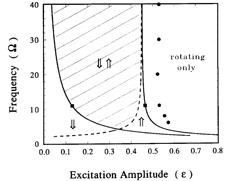
The equation can easily be put in the form of the Mathieu equation, on which there is a wide literature on the properties of stabilization. A diagram of one of the boundaries of stability is shown in [fig-blackburn], sourced from Blackburn and Grnbech-Jensen[1], normalized in terms of non-dimensional physical parameters. The y-axis of frequency is in terms of the ratio of the driven frequency to the natural frequency:
\begin{equation} \Omega = \frac{\omega}{\omega_0}. \label{eq:Omega}\end{equation} The x-axis of excitation amplitude is \begin{equation}\epsilon = \frac{Amr}{I}.\label{eq:epsilon}\end{equation} If the pendulum can be modeled as a point mass, $I=mr^2$ and epsilon simplifies to $\epsilon =\frac{A}{r}$, the ratio of the driven amplitude, to pivot-to-C.o.M. radius. The shaded region indicates stability in both equilibrium orientations, whereas the up and down arrows designate the regions for stability of the hanging and inverted orientations.
Physical Model
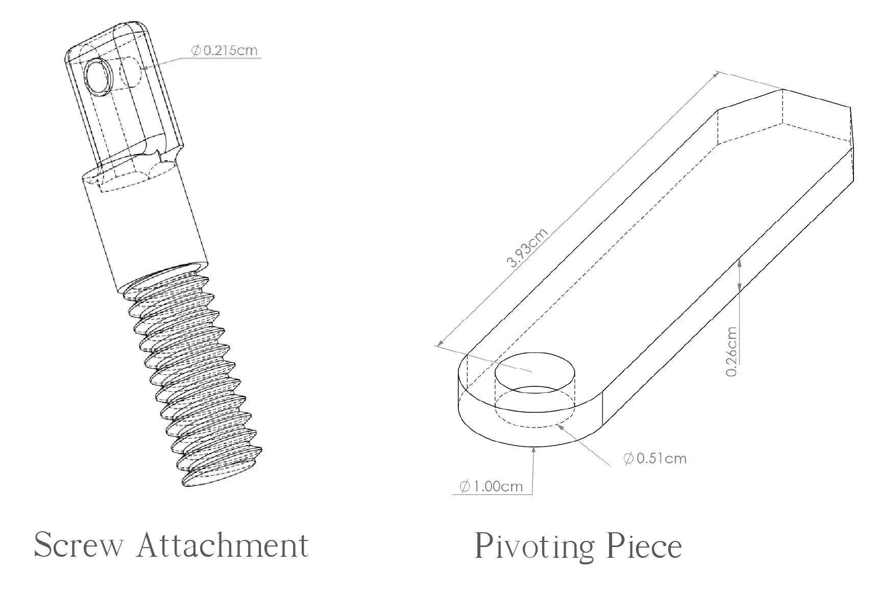
The pendulum model was built in SolidWorks, [fig-stlDiag], and printed in gray resin. It consists of a piece which pivots on a single axis (the ”mass”), and a piece which connects the pivoting piece with the actuator (in this, a speaker cone). The pivoting piece (mass) is made with a hole in which a small bearing (outside diameter: 5mm, inside diameter: 2mm) fits snugly. The two pieces are connected using the bearing and an 8mm x M2 screw and nut. For the actuator, a speaker and amplifier are used. A piece of acrylic, tapped with a 1/4 − 20 thread, has been glued to the speaker head. The amplifier is connected to my laptop via an aux port, and a MATLAB script is used to drive the speaker at a chosen frequency. This provides the sinusoidal oscillations which lead to an inverted stability. The amplitude of oscillations is dependent on the laptop’s output volume and a potentiometer in the amplifier circuit. The size of the pendulum’s mass is limited by the small range of the speaker’s amplitude. Because higher mass requires greater amplitude for an inverted stability, and the limited range of the speaker’s amplitude, the pieces were made quite small. Furthermore, the speaker is unable to drive the higher frequencies at the maximum amplitude, and the weight of the pieces will negatively impact the range. One final issue is that the speaker has a physical limit before it ”bottoms out;” it can only be driven so hard. Despite these considerations, for a pendulum this size the speaker is able to reach the solution space of frequency and amplitude necessary to induce stability.
Though the pendulum differs in shape from the traditional ’mass on a string,’ the rotational inertia can be calculated using SolidWorks to find the moment of inertia of the normal face relative to the axis of rotation, $I_{\text{yy}}$. The rotational inertia is then
\begin{equation}
I = I_{\text{yy}} *\text{depth}*\rho
\end{equation}
where $\rho$, the density, can be computed using the volume from the SolidWorks model in conjunction with the mass measurement from a bench scale of: $m= 1.3155 * 10^{-3} \mathrm{kg}$. The rotational inertia was then found as $I = 6.256*10^{-7}\mathrm{kg\cdot m^2}$.
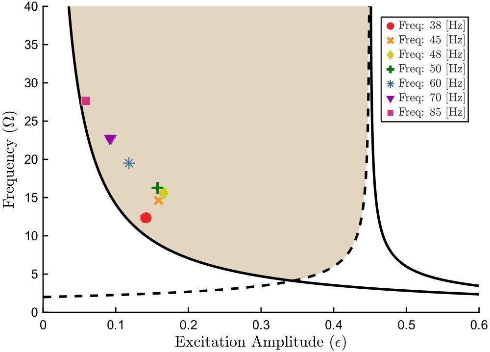
Iterating through a number of driving frequencies, videos of the dynamic stability were recorded with a Photron FastCam R3 at 2000 fps. One video was shot at 5000 fps to achieve a higher temporal resolution of the pendulum oscillations, but 2000 fps was more than adequate to capture the fast and slow behaviors of the pendulum. For each video a point at the tip of the pendulum was tracked using the software tool Tracker, which allowed the extraction of the amplitude of the stable oscillation. The values for the derived amplitudes for each video are below in [tab-parameters], as are the frequency and amplitude in terms of the non-dimensional parameters from Eqs. \ref{eq:Omega}, \ref{eq:epsilon}. Finally, the diagram shown in [fig-blackburn], has been recreated in [fig-experiementalStabilityDiag] and overlaid with values from the video trials. As can be seen, there is excellent argeement between the theoretical and experimental results in regards to dynamic stability.

Response to Perturbation
For each video, we began by letting the pendulum stay in a stable upright configuration for a short time before physically perturbing the pendulum with a screwdriver or ruler, and recording until the pendulum had returned to the upright position. Below is an example of one the videos, overlaid with a portion of the forward-time return to stability to help visualize the pendulum’s motion (recorded at 2000 fps, displayed at 60 fps).
One of the interesting things that can be accomplished with the tracking data is estimating the damping coefficient of the system, via fitting the deflection angle of the pendulum to the differential equation. For this example let’s use the 50 Hz trial, the full video of which can be seen below. As you watch, keep in mind the time-scale of the video. Recorded at 2000 fps, and displayed here at 30 fps, the entire recording takes place in the span of less than 1.35 seconds. If you are interested in seeing any of the other trials they are available here.
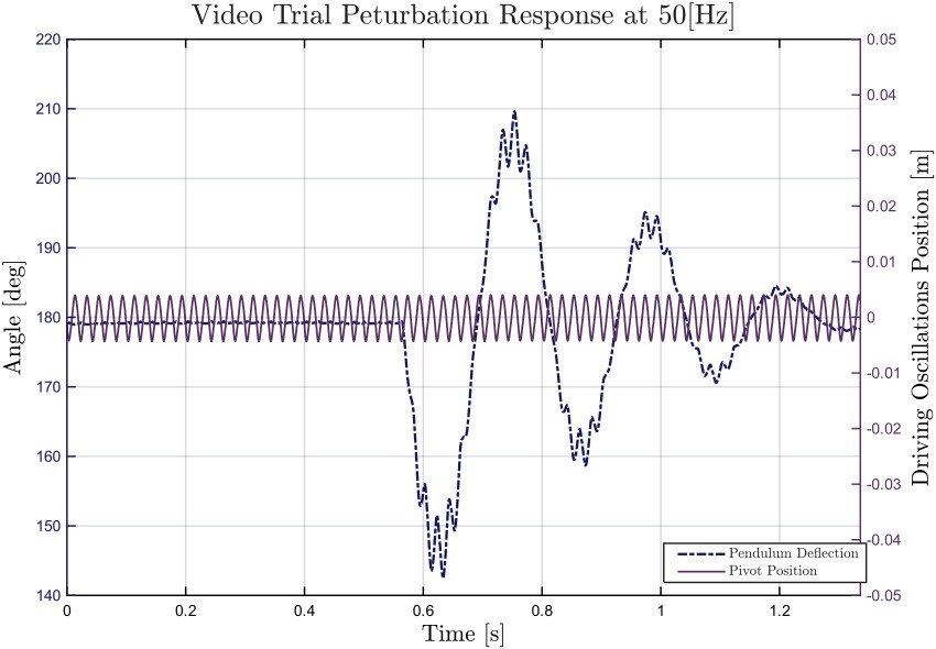
The pendulum deflection angle and the vertical pivot position over the time of the recording is plotted in [fig-50HzAngle], demonstrating the slow and fast motions of the pendulum, respectively. Before we fit the data, let’s make some substitutions to Eq. \ref{eq:DE} so it only includes $\omega_0$, $Q$, $\epsilon$, and $\Omega$ as follows:
\begin{equation}
\ddot{\theta} + \frac{\omega_0}{Q}\dot{\theta} + \big( \epsilon \Omega^2 \omega_0^2 \cos(\Omega \omega_0 t) - \omega_0^2\big)\sin(\theta) = 0 \label{eq:DEsub}
\end{equation}
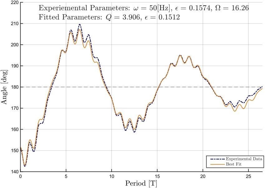
Now, through the power of writing the above as a system of equations in conjunction with MATLAB’s lsqcurvefit() and ode45(), we can fit the experimental data to Eq. \ref{eq:DEsub}. Ideally, we only would want to fit the differential equation by allowing the parameter $Q$ to vary, but generally that provided middling results. By additionally fitting $\epsilon$ and/or $\Omega$ the optimization can be improved. For the 50 Hz example, we’ll take a section starting from just before the greatest deflection, around 0.62 seconds, and limit the section until after a few large oscillations, to about 1.15 seconds. The best fit found via optimizing $Q$ and $\epsilon$, (and setting $\Omega =$ 16.62 based on [tab-parameters]), is shown in [fig-bestfit]. Here the time has been scaled to the period of the small oscillations of the speaker. As displayed in the figure, the best fit parameters include a damping coefficient, $Q =$ 3.906 and, $\epsilon =$ 0.1512, which is near to the derived value of $\epsilon =$ 0.1574. On account of the fact that the experimental data does not perfectly reflect the differential equation (though I did pick a particularly flattering example from the trials), I would surmise that the effect of damping may be more complex than simply being proportional to the velocity. Also, the oscillated pivot via the speaker is near, but not quite, vertical. Instead, it is actually biased about 1-2 degrees from the upright position, and this may account for some of the discrepancies. However, I am rather pleased with how well the data can be fitted overall, as there are bound to be some disparities between the experimental and the theoretical.
Lastly, as a closing thought I must recommend a paper, "On the dynamic stabilization of an inverted pendulum" by Eugene I. Butikov, for a very intuitive explanation of the inverted pendulum's dynamic stability. While most papers focus on the abstract mathematical justifications of stability, Butikov instead gives a very grounded description based on the forces experienced by the pendulum that will be clear to those without a deep background in mathematics.
References
[1] Smith, H. J., J. A. Blackburn, and N. Grnbech-Jensen. "Stability and Hopf bifurcations in an inverted pendulum." Am J Phys 60 (1992): 903-908.
[2] Butikov, Eugene I. "On the dynamic stabilization of an inverted pendulum." American Journal of Physics 69, no. 7 (2001): 755-768.