
For an incompressible, inviscid, 2D flow whose motion is created by a point vortex, how can one create efficient mixing of passive particles? This model of potential flow, while simple, is a useful method for understanding the necessity of a third dimension, here time, to create 'chaos' in the system. By recreating and expanding on the numerical experiments performed in Hassan Aref's 1984 paper: Stirring by chaotic advection, we can establish a greater understanding of potential flow theory, and hopefully create some satisfying images and videos along the way.
It is convenient when dealing with potential flows to work within the complex plane. Using the standard $z=x+iy$, $z$ represents a point in the 2D plane where $x$ is the real axis and $y$ is the imaginary axis. We'll use another complex variable $w$, the complex potential. It is defined as $w=\phi + i \psi$, and is a function of $z$: $f(z)=w$. By nature of satisfying the Cauchy-Riemann equations, the velocity components of the flow are obtained through the derivative of $w$:
\begin{equation}
\frac{dw}{dz} = u -iv,
\end{equation}
where $u$ is the velocity in the x-direction, and $v$ for the y-direction. In all that follows we'll be representing irrotational vortices, which are defined by the following complex potential:
\begin{equation}
w=-\frac{i\Gamma}{2\pi}\ln(z-a),
\label{eq:irr_vort}
\end{equation}
with strength $\Gamma$ (counterclockwise), and position (complex) $a$.

The method of images is a way of satisfying the boundary conditions for singularities within the boundary by placing virtual (image) singularities outside the boundary. The simplest example of this would be a point vortex next to a wall. For potential flow, the boundary condition we must satisfy is no penetration at the wall.
The image vortex in this case is at a position reflected by the wall, that is to say, taking the wall as a line of symmetry. Also of note is that the strength of the image vortex is the same magnitude, but the opposite direction, of the original point vortex.
The experimental setup is an idealized case of stirring devices within a tank, represented by point vortices within a circular 2D bounding contour. Aref specifies that "if an arbitrary number of agitating vortices are held at arbitrarily chosen fixed positions, the advecting flow field gives integrable particle motion and inefficient stirring." Furthermore, even a single stirrer that is permitted to move can produce efficient mixing. As Aref shows, a very simple movement scheme is enough to create chaotic mixing. The simple case that Aref explores in his paper and that is replicated in what follows has been coined as the 'blinking vortex.' This is described as a stirrer that 'blinks' or 'jumps' in between two fixed positions, or equivalently, two stirrers at fixed positions that alternate which of them is on. The function that determines the stirrer position is
\begin{equation}
z(t) = \begin{cases}
+b & (nT \leq t < (n +\frac{1}{2})T), \\
-b & ((n +\frac{1}{2})T \leq t < (n+1)T),
\end{cases}
\label{eq:stirrer_piecewise}
\end{equation}
where $n$ is the set of integers acting as the period counter. $b$, $T$ are constants, and $b<a$ .Let $a$ be the radius of the circular boundary, and $b$ (allowed to be complex) the first position of the stirrer, which will alternate between $+b$ and $-b$. $\Gamma$ is the strength of the stirrer, as defined as a vortex in Eq. \ref{eq:irr_vort}. $t$ is time and $T$ is the period of the stirrer's motion. These are compiled in [tab-params]. In the numerical experiments modeled, $a=1$, $b=0.5$, and $\Gamma=2\pi$. To simplify analysis, the following non-dimensional parameters and variables are introduced.
\begin{gather}
\beta = \frac{b}{a}, \\
\mu = \frac{\Gamma T}{2 \pi a^2}, \\
\tau = \frac{t}{T},
\end{gather}
where $\beta$ represents the normalized position of the stirrer, $\mu$ represents the non-dimensional period of motion, and $\tau$ is the dimensionless time. These are compiled in [tab-dimlessParams]. In what follows, assume $\beta = 0.5$, and $\mu = T$. $T$, and by extension $\mu$, is the parameter varied throughout the following numerical experiments.
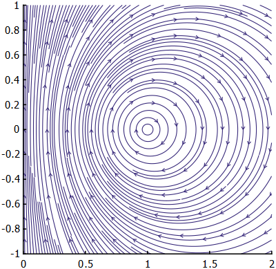
In this particular experimental setup, we do not have to rely on integrating the flow-field as a way to move the particles forward in time. For the case of a single stirrer within a circular boundary, the streamlines upon which particles are advected are circles. For any particle in the flow we can find the center and radius of the circular streamline it lies on and move the particle along the arc as necessary. This is the method used by Aref, which is replicated in this section.
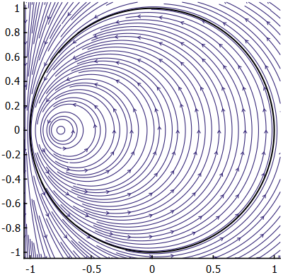
Taking a look at [fig-circBoundary], it is easy to see that the streamlines within (and outside) the boundary are circular. These circles are best described by the Apollonian definition: a set of points $\mathbf{Q}$ with a constant ratio of distances to two foci. For these experiments, the position of the vortex inside the boundary, and the position of the image vortex are the foci. Given the setup in [fig-apolloniusAnim], let $d_1$ be the distance from $P$ to $A$, and $d_2$ be the distance from $P$ to $B$. The ratio of distances $d_1/d_2$ is equal to a constant $k$, for all points on the black circular boundary. But this is not just true for the black boundary, this is true for all the sets of streamlines in the experimental setup, for varying values of $k$.

Here we'll only consider the case during the first half of the stirrer period, defined in Eq. \ref{eq:stirrer_piecewise}, in which the stirrer is at the $+b$ position, as the process for the second half is almost identical. To find the streamline a particle will follow given its initial position, $\zeta_0$, we first calculate $k$, referred to as $\lambda$ in Aref's work, with the following equation
\begin{equation}
k = \left|\frac{\zeta_0-b}{\zeta_0-{a^2}/{b}}\right|.
\end{equation}
Then we can find the center of the Apollonius circle $\zeta_c$ via
\begin{equation}
\zeta_c = \frac{b-k^2a^2/b}{1-k^2},
\end{equation}
and the radius of the Apollonius circle $\rho$ via
\begin{equation}
\rho = \left(\frac{k}{1-k^2}\right) \left|b-\frac{a^2}{b}\right|.
\end{equation}
Now we find the initial angle, $\theta_0$, of the particle relative to the Apollonius circle center by solving
\begin{equation}
\zeta_0-\zeta_c = \rho e^{i\theta_0}
\end{equation}
for $\theta_0$:
\begin{equation}
\theta_0 = -i \ln(\frac{\zeta_0-\zeta_c}{\rho}).
\end{equation}
Then, we can use the function
\begin{equation}
A_{k}(\theta) = \theta - \frac{2k}{1+k^2}\sin(\theta),
\label{eq:A_k}
\end{equation}
which describes the particle's motion in a one-to-one correspondence with $\theta$ (see Aref for derivation), to compute $A_{k}(\theta_0)$. The period of rotation $T_k$ is
\begin{equation}
T_k = \frac{\rho^2}{\Gamma} \frac{1+k^2}{1-k^2},
\end{equation}
and the change in $A_k(\theta)$ is
\begin{equation}
\Delta A_k(\theta) = \frac{\Delta t}{2\pi T_k}.
\end{equation}
Then calculate $A_k(\theta)$ after the advection,
\begin{equation}
A_k(\theta_{t}) = A_k(\theta_0) + \Delta A_k(\theta),
\end{equation}
and finally invert Eq. \ref{eq:A_k} to find the $\theta$ after $\Delta t$ time has passed. The new position of the particle is then
\begin{equation}
\zeta_{t} = \zeta_c + \rho e^{i\theta_t}.
\end{equation}
Using the above procedure we can advect particles, and keeping track of the position of the stirrer, can follow the position of the particles according to the experimental setup.
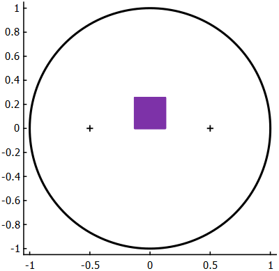
To show the effect of the relevant parameters towards chaotic mixing Aref uses a simulated 'blob' of fluid and advects it forward in time. He creates a square of 10,000 marker particles and simulates the particles until $t=12$ seconds for the following cases: $\beta=0.5,\ \mu=\{0.1,1,2,3\}$. Here we will do the same demonstrations, and a couple additional cases, in video format. The initial position of the particles is shown in [fig-SquareArray]. From the initial positions, we then move each particle forward to its position at every frame based on the equations above, with special attention paid to the position of the stirrer, and keeping track of the particles if the stirrer swaps position between frames. In the following you can see the videos of the experiments and the original work from Aref.
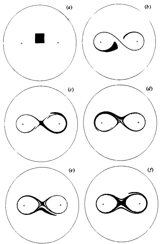

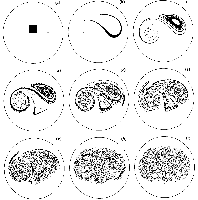

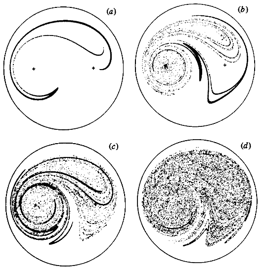

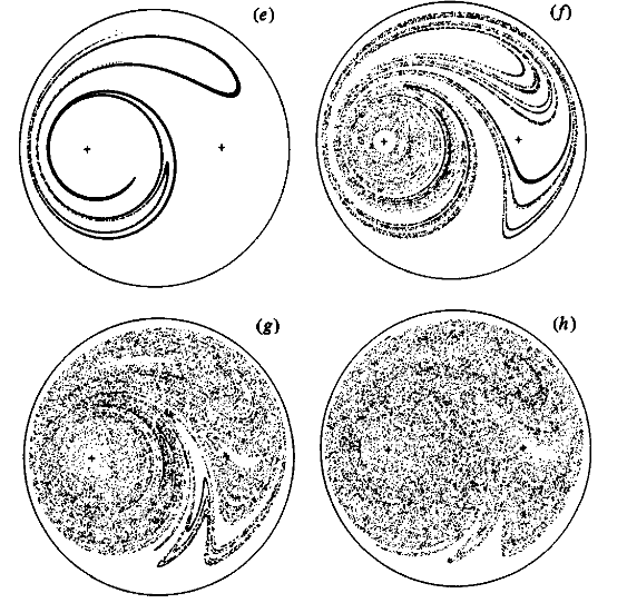


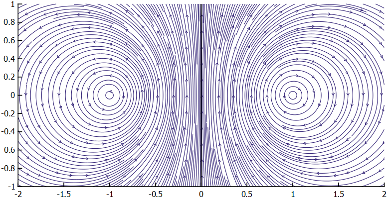
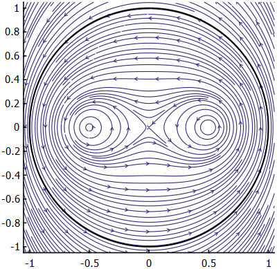
As shown by Aref, we can see that the size of the mixing region, and the chaotic nature of the flow-field, grows with $\mu$. In a slightly more intuitive way, as the time between switching the stirrer position diminishes, the closer the flow tends towards the case in which the two stirrers are running concurrently, the streamlines of which are shown in [fig-bothStirrers].
In the final sections of the paper, Aref discusses some of the interesting features of the experiments. One feature of note are the structures called 'whorls' and 'tendrils', terms borrowed from earlier works on dynamical systems. 'Whorls' appear as winding spirals, seen above in the square array visualization for $\mu$ at 1 and above. 'Tendrils' are described as undulations due to alternating stretching and compressing on the vortices, and can be seen in [fig-Tendrils]. These are created by using a single line of 20,000 starting particles along the y-axis, and instituting the same advection steps as in the previous section. These tendrils arise due to hyperbolic fixed points in which trajectories approach along stable manifolds and leave along unstable manifolds.
Another feature of interest are the 'islands' that appear under the conditions of large $\mu$'s and small $\beta$'s. This corresponds to stirrers very close in to the center of the circle and stirrers swapping on/off at a relatively large time scale. These islands are stable fixed points within the chaotic region where stirring does not occur, which can be seen in [fig-IslandMu4] and [fig-IslandMu3].


The associated MATLAB code can be found on my GitHub. One thing of note, is that many of the plotting functions (which are exported as .svg, then converted to .png/.jpg) rely on the CLI applications "rsvg-convert", "magick" (ImageMagick). These conversion calls from MATLAB will only work properly on a Windows machine, and these programs will need to be added to your PATH in order to be properly called. Additionally, version R2025a or newer is necessary.